Notes for Computer Graphics

学了一学期的计算机图形学，虽然学的不深，OpenGL编程也是浅尝则止，终归算是初步窥得一眼这个领域大体上的景致，想起当初选这门课，是想以后工作了，大抵是不会这么花时间来了解这些东西的了，而这又是我感兴趣想要弄懂弄明白的东西，再有便是想打多些c++代码，总的来说我还是蛮喜欢c++的。

月末是计图期末考试，老师说，有些硬知识还是得考一考的，于是便复习了整学期的ppt，简单地整理出一些笔记

Chapter i when i<5

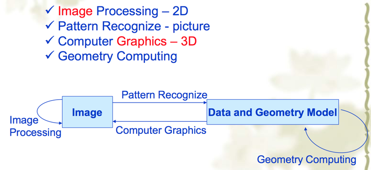
What is CG? — Relative Disciplines
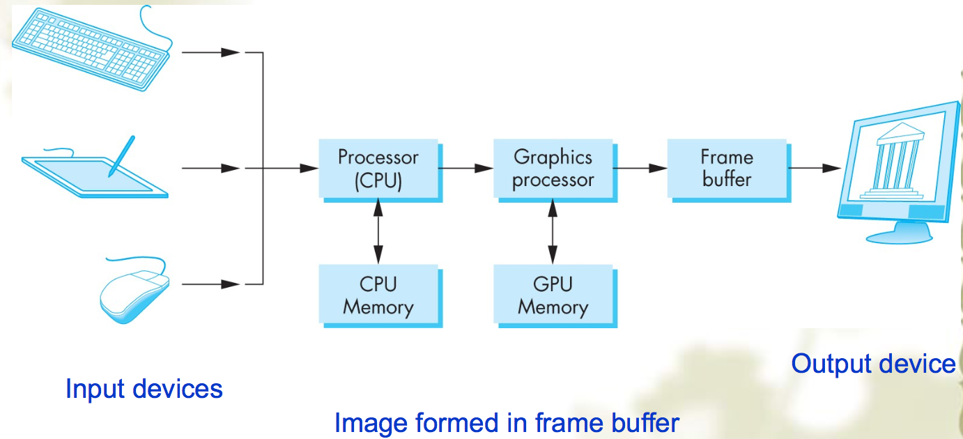
Graphics System
Graphics pipeline
- The Modeling pipeline
- The Rendering pipeline
  - The modeling pipeline only maps vertices between the various spaces
  - All vertices are processed to form an image in frame buffer
Shaders
- Programs used to control GPU

Libraries about OpenGL
- GLU (OpenGL Utility Library)
  - Provides functionality in OpenGL core but avoids having to rewrite code
- GLUT (OpenGL Utility Toolkit)
  - Provides functionality common to all window system
  - Was created long ago and has been unchanged
- FreeGLUT updates GLUT
- GLEW (OpenGL Extension Wrangler Library)
  - Makes it easy to access OpenGL extensions available on a particular system

Dict

To **tessellate** is to make a pattern using identical shapes, creating a consistent pattern like a honeycomb.

About the order of the tranformation matrices

Any combination of the order SRT gives a valid transformation matrix. However, it is pretty common to first scale the object, then rotate it, then translate it:

L = T * R * S

If you do not do it in that order, then a non-uniform scaling will be affected by the previous rotation, making your object look skewed. And the rotation will be affected by the translation, making the final position of your object very different from what the value of the translation would make you expect.

Collision Detection Algorithm

两个包围球或包围盒：其球心距小于半径和
一物所有三角形于另一包围球，若顶点球心距离小于三角形最长边+球半径，则可能，或者三角形外接圆与包围球圆球心距离小于两半径和，则可能
判断两三角形————判断一三角形每个顶点是否在另一个三角形平面的一边，如不在则可能碰撞
交点Q，若以下三不等式成立则Q在三角形$P_1,P_2,P_3$里面
- $N\cdot ((P_1-P_0)\times (Q-P_0)) \gt 0$
- $N\cdot ((P_2-P_1)\times (Q-P_1)) \gt 0$
- $N\cdot ((P_0-P_2)\times (Q-P_2)) \gt 0$

Chapter 5 Lighting and Shading

Current Light Model — Local Lighting Model (LLM)
- consider only lights in the scene, ignore reflected lights
- Three Components:
  - Ambient Light
    - $L_0$ — scene-defined ambient value
    - $L_A$ — individual light contributions from ambient light
    - $C_A$ — material ambient value
    - Total ambient light $A = L_0+\sum_{lights}{(L_A*C_A)}$
    - not care lightPos, viewPos, normals of surface
  - Diffuse Light
    - $L_D$ — light diffuse value
    - $C_D$ — materials diffuse value
    - $D$ — total diffuse light
    - L — light vector
    - N — normal vector
    - $D=\sum_{lights}{L_DC_D(L\cdot N)}$
  - Specular Light
    - K — shininess of the surface — modeled by a cosine function $cos^k(\phi)$
    - R — reflection direction of the light vector
      - $R = L-2(N(N\cdot L))$
    - $C_S$ — materials specular value
    - $S = \sum_{lights}L_SC_S(V\cdot R)^K$
- Use RGB color : $I = (I_R, I_G, I_B)$
- $I = A+D+S$
- prerequisite
  - Normals for each vertex
  - Material for each object
Light
- Light Properties
  - Types of Light Sources
  - Position
  - Directional
  - Spotlight聚光灯 - direction and cutoff
  - Attenuation衰减 - dropoff of values with distance
  - Color for a Light Src in OpenGL
- Types of Light
  - point lights
  - directional/parallel lights
  - spotlights
  - ambient lights
Shading
- Flat & Smooth Shading (OpenGL provide)
  - Smooth shading interpolates vertex colors across the polygon
  - Constant(Flat) Shading
    - Only calculate one point on a polygon(use surface normal) — result is assigned to all other pixels
    - Efficient but often too coarse
  - Discrete Change of Shade
    - Mach band — a stripe found along the edge of two polygons of different shades — occur in constant shading
- Gouraud(Smooth) Shading
  - calculate shading for each vertex of a polygon with its Normal
  - shades of other pixel covered by the polygon is obtained through interpolation
- Phong shading:
  - interpolate the normals across a polygon
  - compute the color for each pixel directly with local lighting model
Computing Light in OpenGL
- Light$(L_R,L_G,L_B)$, Material$(M_R,M_G,M_B)$, then$(L_RM_R,L_GM_G,L_B*M_B)$
- Light$(R_1,G_1,B_1)$, Light$(R_2,G_2,B_2)$, then$(R_1R_2,G_1G_2,B_1*B_2)$
- For all values greater than 1 -> clamped to 1
anisotropic shading各向异性
- deal with objects like hair and CD
Global Illumination
- also considers how light is reflected within a scene
- More complex and realistic
- Main algorithms:
  - Ray tracing
    - Great specular, approx diffuse
  - Radiosity
    - Great diffuse, ignore specular
  - Advanced hybrids: combine them

Chapter 6 Vertices to Fragments

Clipping Algorithms

Line Clipping Algorithms

Cohen-Sutherland
梁友栋-Barsky

1.Cohen-Sutherlan

Two Steps
- Check if the line segment needs to be clipped
- Clip line segment
Cases
- Case 1: Both endpoints of line segment inside all four lines
  - Draw
- Case 2: Both endpoints outside all lines and on the same side of a line
  - Discard
- Case 3: One endpoint inside, one outside
  - Must do at least one intersection
- Case 4: Both outside
  - May have part inside
  - Must do at least one intersection
Using Outcodes
- such as 1001,1000,1010…
- Whether a bit is 1 or 0 depends on the relative position between the endpoint and four lines
- Case
  - outCode(A) = outCode(B) = 0 : Accept
  - outCode(A) = 0 outCode(B) != 0
    - Location of 1 in the outCode(B) determines which edge to intersect with
    - If there are two 1s, we might have to do two intersection
  - outCode(A) & outCode(B) != 0 : reject
  - Neither zero but logical AND yields zero
    - Shorten line segment by intersecting with one sides of window, and then compute outcode of intersection, reexecute algorithm

2.梁友栋-Barsky

参数方程
- $\begin{cases}
  x = x_1 + t(x_2 - x_1)\\
  y = y_1 + t(y_2 - y_1) & 0<=t<=1
  \end{cases}$
- Case ($x_2-x_1>=0$) xL为始边, xR为终边
- Case ($y_2-y_1>=0$) yB为始边, yT为终边
- Otherwise
- Compute $t_1^{‘}, t_1^{‘’}$, then $t_1=max{t_1^{‘}, t_1^{‘’}, 0}$
- $t_2=min{t_2^{‘}, t_2^{‘’}, 0}$
- Result
  - when $t_1<t_2$, the line segment is visible
  - when $t_1>t_2$, the line segment is invisible
- Process to compute $t_1,t_2$
  - $x_L <= (x_2-x_1)*t + x_1 <= xR$
  - $yB <= (y_2-y_1)*t + y_1 <= yT$
  - Simplify it into $t*p_k <= q_k, k=1,2,3,4$
- From the above, we get
  - $p_k<0, t_k$为始边之交点参数
  - $p_k>0, t_k$为终边之交点参数
  - $p_k=0 \text{ && } q_k<0, $则线段完全不可见

Polygon Fill-Area Clipping

for (window_line: window[1-4]){
    for(polygon_line: Polygon[1-n]){
        compute output vertex
    }
    get a sequence of vertices
}
get a final sequence of vertices

Process
- Output vertices that fall on the specific side of the line or intersect with that line

Rasterization: Scan Conversion

Rasterization (scan conversion)
- Determine which pixels that are inside primitive specified by a set of vertices
- Produces a set of fragments
- Fragments have a location(pixel location) and ohter attributes such color and texture coordinates that are determined by interpolating values at vertices
Pixel colors determined later using color, texture, normal and other vertex properties

DDA Algorithm — Scan conversion for line

DDA(Digital Differential Analyzer)

Line equation: $y = m*x+b$

Case

Case $|m|\le 1$
- $x_1\lt x_2$ then $x_{i+1} = x_i + 1, y_{i+1} = y_i + m$
- $x_1\gt x_2$ then $x_{i+1} = x_i - 1, y_{i+1} = y_i - m$

Case $|m|\gt 1$

$y_1\lt y_2$ then $y_{i+1} = y_i + 1, x_{i+1} = x_i + 1/m$

$y_1\gt y_2$ then $y_{i+1} = y_i - 1, x_{i+1} = x_i - 1/m$

line(int x1，int y1，int x2，int y2)
{
    int length, i;
    float dx, dy, x, y;
    length = abs(x2-x1); if(abs(y2-y1) > length) //m>1
    length = abs(y2 - y1);
    dx =(float)(x2 – x1)/length;
    dy =(float)(y2 – y1)/length;
    x = x1 +0.5*sign(dx);
    y = y1 +0.5*sign(dy);
    for(i=1; i <= length; i++) {
        setpixel((int)x,(int)y); 
        x = x + dx;
        y = y + dy;
    }/* for */
}/* line */

Bresenham Algorithm — Scan conversion for line

image_1c2b8lleqbffm3o1o1io2069e9.png-67.1kB

Only discuss the situation when $0\lt |m| \le 1$ and $x_2 \gt x_1$

To decide $y_{i+1} = y_{i}+1 or y_{i+1} = y_i$, according to the distance of AB and the distance of BC
let d1 = BC, d2 = AB
- if d1>d2, get the upper point
- if d1<d2, get the lower point
Something magic….
- $p_i = \Delta x*(d_1-d_2)=…$
- …After a lot of computation, we finally get
- $p_{i+1} = p_i + 2\Delta y - 2\Delta *(y_{i+1}-y_i)$
- Hence, at every step, we just compute the value of $p_i$ according to the previous value of p, and
  - if $p_i>0 $ -> $ d_1-d_2>0$
  - if $p_i<0 $ -> $ d_1-d_2<0$
- THe end
  - $p_1 = 2*\Delta y - \Delta x$
  - $x_{i+1} = x_{i}+1$
  - $y_{i+1} = \begin{cases} y_i+1&\text{if } p_i>0 \\ y_i & \text{if } p_i\le0 \end{cases}$
  - $p_{i+1} = \begin{cases} p_i+2(\Delta y-\Delta x)&\text{if } p_i>0 \\ p_i+2\Delta y & \text{if } p_i\le0 \end{cases}$

Scan Conversion for Polygon

A **scan line** (also **scanline**) is one line, or row, in a raster scanning pattern, such as a line of video on a cathode ray tube (CRT) display of a television set or computer monitor

Step
- First find out the scanlines that intercept with the polygon. Calculate the overlapping segments
- For each scanline from top to botton, set the pixels in the segment
Definition of Fragments
- If there are exactly two edges that meet a scan line of pixels, we need to determine the color of all pixels between the two edge pixels on the scan line
- These pixels are called of a fragment
- Two steps:
  - 求交
  - 排序 according to the x-coordinates
  - if intersect with a vertex:
    - if it is a extreme point, then it counts 2 points
    - else it counts 1 point

Hidden-Surface Removal

The z-Buffer Algorithm
- Depth Buffer same as Frame Buffer
- saving the distance of the closest intersection
The Painter’s Algorithm
- Rendering from back to front of the polygons
- depth sort for all polygons
- dividing the polygon into two parts

Antianliasing

Compute the overlapping proportions of the lines and the nearby pixel squares.
Suppose that the overlapping proportion of a certain pixel is $\alpha$, the new pixel_color is then set to

$\alpha \times currentColor + (1-\alpha) \times existingColor$

Line Antianliasing
Polygon Antianliasing

Color Model

Color
- Hue(色调) or chroma
- Saturation(饱和度) 掺入白光的多少
- Luminance(明亮度) 光的能量大小
Color Model
- RGB — cube for screen
  - Luminance = 0.30red + 0.59green + 0.11*blue
- CMYK — cube for printer
- HSV — cone(圆锥体) for artist
  - Hue = angle
  - Saturation = radius
  - Value = height
- HLS — double cone for artist on painting

!!!Emissive vs Transmissive Color

Emissive
- From screen
- RGB emissive model - additive colors
Transmissive
- From inks
- CMYK transmissive model - subtractive color